Comparison with the decider package

In this vignette we want to compare the combination design implemented in crmPack and explained in this vignette with the implementation in the decider package (Schroeter 2023). Please note that the decider package is not available on CRAN, therefore this vignette is precomputed from a source file that runs with decider installed.

Example

We are going to use the example as described in the decider vignette here:

• Three arms:
  • Arm A: monotherapy of compound 1
  • Arm B: combination of compound 1 and compound 2
  • Arm C: historical data from compound 2
• Arm B can start when certain doses of Arm A have been cleared
• Logistic log-normal models for compound 1 and compound 2
• Target interval is 16-33% DLT rate
• Prior specification
  • uniform prior for the correlation between intercept and log-slope in the logistic log-normal model
  • for the hyper-means (i.e. mean of parameters across trials)
  • between-trial heterogeneity (i.e. standard deviation of parameters across trials)

Using decider

library(decider)

This is the data from the historical Arm C:

historical_data <- list(
  dose1 = c(0, 0, 0, 0, 0),
  dose2 = c(2, 4, 8, 12, 16),
  n.pat = c(3, 3, 3, 9, 12),
  n.dlt = c(0, 0, 0, 1, 2),
  trial = c("H1", "H1", "H1", "H1", "H1")
)

The monotherapy dose grid for Arm A is:

d1 <- c(0.1, 0.2, 0.4, 0.8, 1.6, 2.4, 3.6, 5, 6)

The dose grid for compound 2 in Arm B is more sparse:

d2 <- c(8, 12)

The overall dose grid for combination Arm B is therefore:

doses_of_interest <- rbind(
  c(d1, rep(d1, times = length(d2))),
  c(rep(0, length(d1)), rep(d2, each = length(d1)))
)

The reference doses to be used in the models are:

dose_ref1 <- 6
dose_ref2 <- 12

We further need to specify the arms and types of the arms as follows:

trials_of_interest <- c("A", "B")
types_of_interest <- c("mono1", "combi")

The prior for the hypermeans is specified like this:

#                Parameter   Mean         SD
prior_mu <- list(
  mu_a1 = c(logit(0.33), 2),
  mu_b1 = c(0, 1), # standard normal
  mu_a2 = c(logit(0.33), 2),
  mu_b2 = c(0, 1), # standard normal
  mu_eta = c(0, 1.121)
)

The prior mean for $\mu_{\alpha_{1}}$ is set to $\text{logit}(0.33)$, which implies that we assume the reference dose has a prior median DLT rate of 33%.

Note that we use a normal prior here on the interaction parameter $\eta$, thus allowing both positive and negative interactions. The standard deviation is set such that $\exp(1.96 \cdot 1.121) \approx 9$, thus allowing for a 95% prior interval of $[1 / 9, 9]$ for the odds changes for a DLT at the reference dose. So $1.121 = \log(9) / z_{0.975}$.

The prior for the between-trial heterogeneity parameters is specified like this:

#                 Parameter    Mean        SD
prior_tau <- list(
  tau_a1 = c(log(0.25), log(2) / 1.96),
  tau_b1 = c(log(0.125), log(2) / 1.96),
  tau_a2 = c(log(0.25), log(2) / 1.96),
  tau_b2 = c(log(0.125), log(2) / 1.96),
  tau_eta = c(log(0.125), log(2) / 1.96)
)

These are all the log normal prior parameters for the corresponding $\tau$ parameters. These are all “moderate” degrees of heterogeneity, according to Neuenschwander et al. (2014).

Then we look at the following scenario, where two cohorts of patients are available from Arm A:

scenario1 <- list(
  dose1 = c(0.1, 0.2),
  dose2 = c(0, 0),
  n.pat = c(3, 3),
  n.dlt = c(0, 1),
  trial = c("A", "A")
)

We note that the trial specification here needs to match the name used in trials_of_interest above.

Now we can call the scenario function:

result1 <- scenario_jointBLRM(
  data = scenario1,
  historical.data = historical_data,
  doses.of.interest = doses_of_interest,
  dose.ref1 = dose_ref1,
  dose.ref2 = dose_ref2,
  trials.of.interest = trials_of_interest,
  types.of.interest = types_of_interest,
  prior.mu = prior_mu,
  prior.tau = prior_tau,
  seed = 3819
)

We can look at the results:

result1
#> $`trial-A`
#>          mean      sd  q.2.5%   q.50% q.97.5% P([0,0.16)) P([0.16,0.33))
#> 0.1+0 0.11479 0.10869 0.00311 0.08149 0.40243     0.74108        0.20509
#> 0.2+0 0.15362 0.12839 0.00681 0.11868 0.47993     0.61939        0.27436
#> 0.4+0 0.20692 0.15483 0.01315 0.17076 0.58171     0.47247        0.32265
#> 0.8+0 0.27562 0.18745 0.02261 0.23940 0.70550     0.33297        0.32360
#> 1.6+0 0.35580 0.22114 0.03411 0.32326 0.82755     0.22619        0.28467
#> 2.4+0 0.40489 0.23848 0.04152 0.37742 0.88451     0.18058        0.25176
#> 3.6+0 0.45346 0.25275 0.04956 0.43407 0.92687     0.14457        0.22160
#> 5+0   0.49144 0.26178 0.05658 0.48177 0.95107     0.12236        0.19710
#> 6+0   0.51177 0.26580 0.06038 0.50800 0.96129     0.11191        0.18482
#>       P([0.33,1])
#> 0.1+0     0.05383
#> 0.2+0     0.10625
#> 0.4+0     0.20488
#> 0.8+0     0.34343
#> 1.6+0     0.48914
#> 2.4+0     0.56766
#> 3.6+0     0.63383
#> 5+0       0.68054
#> 6+0       0.70327
#> 
#> $`trial-B`
#>           mean      sd  q.2.5%   q.50% q.97.5% P([0,0.16)) P([0.16,0.33))
#> 0.1+8  0.18532 0.12574 0.02792 0.15549 0.50891     0.51642        0.35703
#> 0.2+8  0.21997 0.14221 0.03572 0.18739 0.57802     0.41292        0.39155
#> 0.4+8  0.26694 0.16307 0.04672 0.23216 0.66265     0.30404        0.39703
#> 0.8+8  0.32790 0.18837 0.06055 0.29352 0.75850     0.20644        0.36283
#> 1.6+8  0.40083 0.21637 0.07448 0.37067 0.85505     0.13707        0.29704
#> 2.4+8  0.44638 0.23299 0.08127 0.42218 0.90297     0.11115        0.25545
#> 3.6+8  0.49155 0.24974 0.08260 0.47743 0.94130     0.09733        0.21504
#> 5+8    0.52620 0.26418 0.07843 0.52496 0.96383     0.09504        0.18686
#> 6+8    0.54406 0.27297 0.07261 0.55181 0.97352     0.09740        0.17310
#> 0.1+12 0.22334 0.12679 0.05283 0.19699 0.54017     0.36499        0.45491
#> 0.2+12 0.25637 0.14136 0.06204 0.22759 0.60438     0.27993        0.46306
#> 0.4+12 0.30120 0.16029 0.07387 0.27114 0.68231     0.19820        0.43482
#> 0.8+12 0.35946 0.18418 0.08771 0.32932 0.77416     0.13208        0.36929
#> 1.6+12 0.42916 0.21272 0.09821 0.40303 0.86742     0.09211        0.28463
#> 2.4+12 0.47244 0.23171 0.09767 0.45369 0.91511     0.08355        0.23692
#> 3.6+12 0.51454 0.25346 0.08738 0.50860 0.95252     0.08684        0.19640
#> 5+12   0.54545 0.27432 0.06937 0.55594 0.97407     0.10030        0.16967
#> 6+12   0.56046 0.28749 0.05723 0.58262 0.98268     0.11168        0.15580
#>        P([0.33,1])
#> 0.1+8      0.12655
#> 0.2+8      0.19553
#> 0.4+8      0.29893
#> 0.8+8      0.43073
#> 1.6+8      0.56589
#> 2.4+8      0.63340
#> 3.6+8      0.68763
#> 5+8        0.71810
#> 6+8        0.72950
#> 0.1+12     0.18010
#> 0.2+12     0.25701
#> 0.4+12     0.36698
#> 0.8+12     0.49863
#> 1.6+12     0.62326
#> 2.4+12     0.67953
#> 3.6+12     0.71676
#> 5+12       0.73003
#> 6+12       0.73252

For each trial of interest, the posterior toxicities previously designated to be of interest are shown.

The public scenario helper returns these posterior summaries, but not the underlying parameter draws. For the parameter-level comparison below, we call the same internal sampler with the same data, settings, and internal seed used by scenario_jointBLRM(). Thus, decider_samples contains the draws from which the summaries in result1 were calculated.

decider_data <- list(
  dose1 = c(historical_data$dose1, scenario1$dose1),
  dose2 = c(historical_data$dose2, scenario1$dose2),
  n.pat = c(historical_data$n.pat, scenario1$n.pat),
  n.dlt = c(historical_data$n.dlt, scenario1$n.dlt),
  trial = c(historical_data$trial, scenario1$trial)
)
decider_trial <- factor(decider_data$trial)
decider_study_index <- c(
  A = match("A", levels(decider_trial)),
  B = nlevels(decider_trial) + 1L,
  C = match("H1", levels(decider_trial))
)

set.seed(3819)
decider_internal_seed <- sample.int(.Machine$integer.max, 1)
decider_samples <- decider:::sampling_jointBLRM(
  dose1 = decider_data$dose1,
  dose2 = decider_data$dose2,
  dose.ref1 = dose_ref1,
  dose.ref2 = dose_ref2,
  n.pat = decider_data$n.pat,
  n.dlt = decider_data$n.dlt,
  n.study = as.integer(decider_trial),
  MAP.prior = TRUE,
  prior.mu = prior_mu,
  prior.tau = prior_tau,
  iter = 26000,
  warmup = 1000,
  refresh = 0,
  adapt_delta = 0.8,
  max_treedepth = 15,
  chains = 4,
  seed = decider_internal_seed
)

Under the hood, the implementation works as follows:

• post_tox_jointBLRM() is called to sample from the posterior, which in turn uses
• sampling_jointBLRM() which then calls rstan::sampling() on
• stanmodels$jointBLRM which is the constant Stan model sourced from
• jointBLRM.stan

So we can compare this with the implementation in crmPack which is based on JAGS.

Using crmPack

Now we are going to define the same design and scenario in crmPack.

We start with the monotherapy model for compound 1:

library(crmPack)

mono_model1 <- LogisticLogNormal(
  mean = c(logit(0.33), 0),
  cov = diag(c(2, 1)^2),
  ref_dose = dose_ref1
)

And for compound 2 the same:

mono_model2 <- LogisticLogNormal(
  mean = c(logit(0.33), 0),
  cov = diag(c(2, 1)^2),
  ref_dose = dose_ref2
)

Then we define the combination model:

combo_model <- TwoDrugsCombo(
  list(
    compound1 = mono_model1,
    compound2 = mono_model2
  ),
  gamma = 0, # prior mean for the interaction parameter
  tau = 1 / (1.121^2) # prior precision for the interaction parameter
)

We define the historical data which is already available:

hist_data_comp2 <- Data(
  x = rep(historical_data$dose2, historical_data$n.pat),
  y = unlist(Map(
    function(n_pat, n_dlt) {
      c(rep(0, n_pat - n_dlt), rep(1, n_dlt))
    },
    historical_data$n.pat,
    historical_data$n.dlt
  )),
  doseGrid = historical_data$dose2
)
hist_data_comp2

Evaluable participants to-date

ID	Cohort	Dose	DLT?
1	1	2	FALSE
2	1	2	FALSE
3	1	2	FALSE
4	2	4	FALSE
5	2	4	FALSE
6	2	4	FALSE
7	3	8	FALSE
8	3	8	FALSE
9	3	8	FALSE
10	4	12	FALSE
11	4	12	FALSE
12	4	12	FALSE
13	4	12	FALSE
14	4	12	FALSE
15	4	12	FALSE
16	4	12	FALSE
17	4	12	FALSE
18	4	12	TRUE
19	5	16	FALSE
20	5	16	FALSE
21	5	16	FALSE
22	5	16	FALSE
23	5	16	FALSE
24	5	16	FALSE
25	5	16	FALSE
26	5	16	FALSE
27	5	16	FALSE
28	5	16	FALSE
29	5	16	TRUE
30	5	16	TRUE

The dose grid is 2, 4, 8, 12 and 16.

We are going to use simple rules here (they are not relevant for the current scenario comparison):

my_stopping <- StoppingMinPatients(nPatients = 50)
my_increments <- IncrementsRelative(0, 2)
myNextBest <- NextBestNCRM(
  target = c(0.16, 0.33),
  overdose = c(0.33, 1),
  max_overdose_prob = 0.25
)
my_cohort_size <- CohortSizeConst(size = 3)
my_increments_combo <- IncrementsComboOneDrugOnly()

Then we define the design arms accordingly:

designArmA <- DesignArm(
  "A",
  design = Design(
    data = Data(doseGrid = d1),
    startingDose = d1[1],
    model = mono_model1,
    stopping = my_stopping,
    increments = my_increments,
    nextBest = myNextBest,
    cohort_size = my_cohort_size
  )
)

designArmB <- DesignArm(
  "B",
  design = DesignCombo(
    data = DataCombo(doseGrid = list(compound1 = d1, compound2 = c(0, d2))),
    startingDose = c(compound1 = d1[1], compound2 = 0),
    model = combo_model,
    stopping = my_stopping,
    increments = my_increments_combo,
    nextBest = myNextBest,
    cohort_size = my_cohort_size
  ),
  open_when = ArmMinDoseCondition("A", min_dose = d1[2])
)

designArmC <- HistoricalArm(
  "C",
  data = hist_data_comp2,
  model = mono_model2
)

Now we can define the hierarchical design:

design_hierarchical <- HierarchicalDesign(
  designArmA,
  designArmB,
  designArmC,
  exchangeable_parameters = list(
    comp1_intercept = list(
      A = "alpha0",
      B = "alpha0[1]"
    ),
    comp1_slope = list(
      A = "alpha1",
      B = "alpha1[1]"
    ),
    comp2_intercept = list(
      B = "alpha0[2]",
      C = "alpha0"
    ),
    comp2_slope = list(
      B = "alpha1[2]",
      C = "alpha1"
    ),
    eta = list(
      B = "eta"
    )
  ),
  pool_correlations = list(
    comp1 = c("comp1_intercept", "comp1_slope"),
    comp2 = c("comp2_intercept", "comp2_slope")
  ),
  pool_priors = list(
    comp1_intercept = list(
      mu = prior_mu$mu_a1,
      tau = prior_tau$tau_a1
    ),
    comp1_slope = list(
      mu = prior_mu$mu_b1,
      tau = prior_tau$tau_b1
    ),
    comp2_intercept = list(
      mu = prior_mu$mu_a2,
      tau = prior_tau$tau_a2
    ),
    comp2_slope = list(
      mu = prior_mu$mu_b2,
      tau = prior_tau$tau_b2
    ),
    eta = list(
      mu = prior_mu$mu_eta,
      tau = prior_tau$tau_eta
    )
  )
)

The interaction parameter is included in its own exchangeable pool. Thus each combination arm has a separate interaction parameter $\eta_j$, conditionally distributed as

$$\eta_j \mid \mu_\eta, \tau_\eta \sim \textrm{Normal}(\mu_\eta, \tau_\eta^2),$$

with the same hyperpriors for $\mu_\eta$ and $\tau_\eta$ as in decider. A one-member pool is used here because there is only one combination arm; with multiple combination arms the same definition gives each arm its own interaction parameter while allowing exchangeable borrowing between them.

Note that each entry in pool_correlations can correlate exactly two scalar exchangeable parameter pools. In this example, comp1 correlates the compound 1 intercept pool with the compound 1 slope pool, and comp2 does the same for compound 2. Correlated blocks with three or more parameters are not currently supported.

Then we define the scenario:

scenario_hierarchical <- HierarchicalData(
  A = Data(
    x = c(0.1, 0.1, 0.1, 0.2, 0.2, 0.2),
    y = c(0, 0, 0, 0, 0, 1),
    doseGrid = designArmA@design@data@doseGrid
  ),
  B = designArmB@design@data,
  C = designArmC@design@data
)

And then we can use the scenario() function:

result1CrmPack <- scenario(
  design_hierarchical,
  data = scenario_hierarchical,
  mcmcOptions = McmcOptions(
    burnin = 20000,
    step = 2,
    samples = 100000,
    rng_kind = "Mersenne-Twister",
    rng_seed = 3819
  )
)

We can look at the fit results:

result1CrmPack$fit
#> $A
#>   dose    middle       lower     upper
#> 1  0.1 0.1145638 0.003242997 0.4039016
#> 2  0.2 0.1531443 0.006965511 0.4791348
#> 3  0.4 0.2061103 0.013046402 0.5797054
#> 4  0.8 0.2743383 0.021845606 0.7050774
#> 5  1.6 0.3538963 0.033114229 0.8242544
#> 6  2.4 0.4025788 0.040632531 0.8818548
#> 7  3.6 0.4507303 0.048607949 0.9250483
#> 8  5.0 0.4883849 0.055278969 0.9497937
#> 9  6.0 0.5085354 0.059025056 0.9600121
#> 
#> $B
#>    compound1 compound2    middle       lower     upper
#> 1        0.1         0 0.1182987 0.001874605 0.4559461
#> 2        0.2         0 0.1555321 0.004608167 0.5345317
#> 3        0.4         0 0.2059665 0.010066603 0.6294228
#> 4        0.8         0 0.2712659 0.018552209 0.7343474
#> 5        1.6         0 0.3492500 0.030239089 0.8374834
#> 6        2.4         0 0.3980527 0.037350322 0.8877980
#> 7        3.6         0 0.4469119 0.045289913 0.9272576
#> 8        5.0         0 0.4853478 0.052104606 0.9506019
#> 9        6.0         0 0.5059501 0.055713251 0.9606872
#> 10       0.1         8 0.1848912 0.027797053 0.5074243
#> 11       0.2         8 0.2193303 0.035647160 0.5764916
#> 12       0.4         8 0.2660168 0.046325986 0.6597510
#> 13       0.8         8 0.3265623 0.059819665 0.7575669
#> 14       1.6         8 0.3990081 0.074217951 0.8547246
#> 15       2.4         8 0.4442954 0.080466594 0.9027538
#> 16       3.6         8 0.4892381 0.081642768 0.9410320
#> 17       5.0         8 0.5237206 0.077055551 0.9637166
#> 18       6.0         8 0.5415186 0.071112153 0.9732953
#> 19       0.1        12 0.2228088 0.052696578 0.5386444
#> 20       0.2        12 0.2556630 0.061864866 0.6008869
#> 21       0.4        12 0.3002409 0.073471361 0.6793323
#> 22       0.8        12 0.3581414 0.087348039 0.7727541
#> 23       1.6        12 0.4274556 0.098385029 0.8673500
#> 24       2.4        12 0.4705309 0.097504585 0.9144013
#> 25       3.6        12 0.5124794 0.086888993 0.9519413
#> 26       5.0        12 0.5433086 0.069807168 0.9736904
#> 27       6.0        12 0.5583265 0.056910280 0.9823670
#> 
#> $C
#>   dose     middle        lower     upper
#> 1    2 0.02460650 4.793384e-06 0.1133971
#> 2    4 0.03868410 1.752571e-04 0.1404200
#> 3    8 0.06999088 5.738939e-03 0.1855041
#> 4   12 0.11073085 2.753790e-02 0.2435263
#> 5   16 0.16418890 4.374777e-02 0.3587250

We can also check the probabilities to be in target and overdosing intervals:

result1CrmPack$next_best$A$probs
#>       dose  target overdose
#>  [1,]  0.1 0.20034  0.05460
#>  [2,]  0.2 0.27280  0.10590
#>  [3,]  0.4 0.32488  0.20156
#>  [4,]  0.8 0.32324  0.34144
#>  [5,]  1.6 0.28236  0.48714
#>  [6,]  2.4 0.25191  0.56363
#>  [7,]  3.6 0.22161  0.63034
#>  [8,]  5.0 0.19782  0.67646
#>  [9,]  6.0 0.18614  0.69891
result1CrmPack$next_best$B$probs
#>    compound1 compound2 target_prob overdose_prob not_eligible
#> 1        0.1         0     0.19051       0.07283        FALSE
#> 2        0.2         0     0.24700       0.12309        FALSE
#> 3        0.4         0     0.29509       0.20807        FALSE
#> 4        0.8         0     0.30610       0.33237         TRUE
#> 5        1.6         0     0.27802       0.47361         TRUE
#> 6        2.4         0     0.25074       0.55132         TRUE
#> 7        3.6         0     0.22075       0.62031         TRUE
#> 8        5.0         0     0.19779       0.66861         TRUE
#> 9        6.0         0     0.18538       0.69285         TRUE
#> 10       0.1         8     0.35555       0.12578        FALSE
#> 11       0.2         8     0.39134       0.19427        FALSE
#> 12       0.4         8     0.39878       0.29627         TRUE
#> 13       0.8         8     0.36393       0.42774         TRUE
#> 14       1.6         8     0.29811       0.56336         TRUE
#> 15       2.4         8     0.25635       0.63029         TRUE
#> 16       3.6         8     0.21624       0.68399         TRUE
#> 17       5.0         8     0.18734       0.71495         TRUE
#> 18       6.0         8     0.17439       0.72623         TRUE
#> 19       0.1        12     0.45577       0.17785        FALSE
#> 20       0.2        12     0.46200       0.25568         TRUE
#> 21       0.4        12     0.43539       0.36440         TRUE
#> 22       0.8        12     0.37159       0.49499         TRUE
#> 23       1.6        12     0.28659       0.61978         TRUE
#> 24       2.4        12     0.23968       0.67531         TRUE
#> 25       3.6        12     0.19992       0.71250         TRUE
#> 26       5.0        12     0.17059       0.72856         TRUE
#> 27       6.0        12     0.15689       0.73076         TRUE

Comparison of parameter posteriors

The toxicity summaries at different doses are strongly dependent because they are all transformations of the same small set of model parameters. We therefore compare those parameter posteriors directly. The slopes are shown on their positive, natural scale: decider stores their logarithms, whereas crmPack stores the exponentiated slopes.

crm_samples_A <- armSamples(result1CrmPack$samples, "A")
crm_samples_B <- armSamples(result1CrmPack$samples, "B")
crm_samples_C <- armSamples(result1CrmPack$samples, "C")

# Thin only for plotting; all retained draws are still used in the tables.
n_plot_draws <- 5000L
decider_plot_index <- unique(round(seq(
  1,
  nrow(decider_samples),
  length.out = min(n_plot_draws, nrow(decider_samples))
)))
crm_plot_index <- unique(round(seq(
  1,
  length(crm_samples_A@data$alpha0),
  length.out = min(n_plot_draws, length(crm_samples_A@data$alpha0))
)))

parameter_labels <- c(
  "Arm A: compound 1 intercept",
  "Arm A: compound 1 slope",
  "Arm B: compound 1 intercept",
  "Arm B: compound 1 slope",
  "Arm B: compound 2 intercept",
  "Arm B: compound 2 slope",
  "Arm B: interaction",
  "Arm C: compound 2 intercept",
  "Arm C: compound 2 slope"
)

decider_parameter_draws <- data.frame(
  implementation = "decider",
  parameter = rep(parameter_labels, each = length(decider_plot_index)),
  value = c(
    decider_samples[
      decider_plot_index,
      sprintf("log_ab[%i,1]", decider_study_index["A"])
    ],
    exp(decider_samples[
      decider_plot_index,
      sprintf("log_ab[%i,2]", decider_study_index["A"])
    ]),
    decider_samples[
      decider_plot_index,
      sprintf("log_ab[%i,1]", decider_study_index["B"])
    ],
    exp(decider_samples[
      decider_plot_index,
      sprintf("log_ab[%i,2]", decider_study_index["B"])
    ]),
    decider_samples[
      decider_plot_index,
      sprintf("log_ab[%i,3]", decider_study_index["B"])
    ],
    exp(decider_samples[
      decider_plot_index,
      sprintf("log_ab[%i,4]", decider_study_index["B"])
    ]),
    decider_samples[
      decider_plot_index,
      sprintf("log_ab[%i,5]", decider_study_index["B"])
    ],
    decider_samples[
      decider_plot_index,
      sprintf("log_ab[%i,3]", decider_study_index["C"])
    ],
    exp(decider_samples[
      decider_plot_index,
      sprintf("log_ab[%i,4]", decider_study_index["C"])
    ])
  )
)

crm_parameter_draws <- data.frame(
  implementation = "crmPack",
  parameter = rep(parameter_labels, each = length(crm_plot_index)),
  value = c(
    crm_samples_A@data$alpha0[crm_plot_index],
    crm_samples_A@data$alpha1[crm_plot_index],
    crm_samples_B@data$alpha0[crm_plot_index, 1],
    crm_samples_B@data$alpha1[crm_plot_index, 1],
    crm_samples_B@data$alpha0[crm_plot_index, 2],
    crm_samples_B@data$alpha1[crm_plot_index, 2],
    crm_samples_B@data$eta[crm_plot_index],
    crm_samples_C@data$alpha0[crm_plot_index],
    crm_samples_C@data$alpha1[crm_plot_index]
  )
)

parameter_draws <- rbind(decider_parameter_draws, crm_parameter_draws)
parameter_draws$implementation <- factor(
  parameter_draws$implementation,
  levels = c("decider", "crmPack")
)
parameter_draws$parameter <- factor(
  parameter_draws$parameter,
  levels = parameter_labels
)

First we compare the parameters for the two monotherapy arms:

ggplot2::ggplot(
  parameter_draws[grepl("^Arm [AC]", parameter_draws$parameter), ],
  ggplot2::aes(
    x = value,
    colour = implementation,
    fill = implementation
  )
) +
  ggplot2::geom_density(alpha = 0.15, linewidth = 0.6) +
  ggplot2::facet_wrap(ggplot2::vars(parameter), scales = "free", ncol = 2) +
  ggplot2::labs(
    x = NULL,
    y = "Posterior density",
    colour = NULL,
    fill = NULL
  ) +
  ggplot2::theme_minimal() +
  ggplot2::theme(legend.position = "top")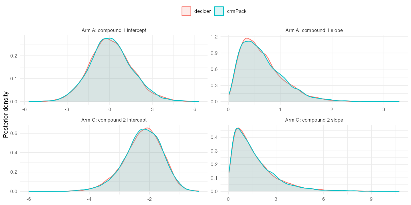

plot of chunk unnamed-chunk-27

And then the parameters for the combination arm, including the interaction parameter:

ggplot2::ggplot(
  parameter_draws[grepl("^Arm B", parameter_draws$parameter), ],
  ggplot2::aes(
    x = value,
    colour = implementation,
    fill = implementation
  )
) +
  ggplot2::geom_density(alpha = 0.15, linewidth = 0.6) +
  ggplot2::facet_wrap(ggplot2::vars(parameter), scales = "free", ncol = 2) +
  ggplot2::labs(
    x = NULL,
    y = "Posterior density",
    colour = NULL,
    fill = NULL
  ) +
  ggplot2::theme_minimal() +
  ggplot2::theme(legend.position = "top")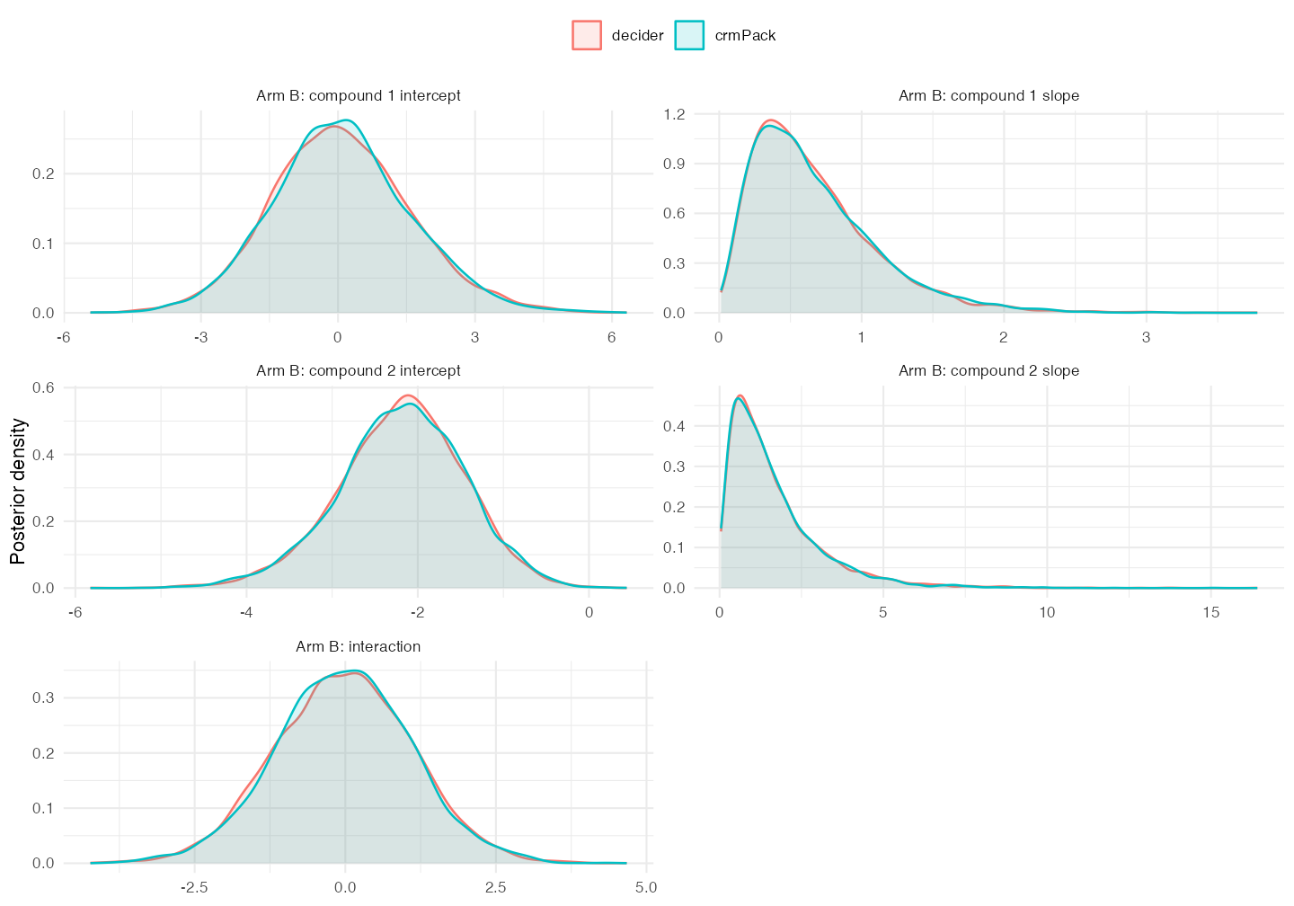

plot of chunk unnamed-chunk-28

Monte Carlo uncertainty of the differences

Overlapping densities alone cannot establish that two posterior distributions are equivalent. We therefore calculate chain-aware Monte Carlo standard errors (MCSEs) for the quantities compared below. The four Stan chains are kept separate; crmPack currently uses one JAGS chain. For each implementation, posterior::mcse_mean() accounts for serial autocorrelation through the bulk effective sample size. Because the Stan and JAGS fits are independent, the MCSE of their difference is

$$\operatorname{MCSE}(\hat\theta_{\text{decider}} - \hat\theta_{\text{crmPack}}) = \sqrt{\operatorname{MCSE}(\hat\theta_{\text{decider}})^2 + \operatorname{MCSE}(\hat\theta_{\text{crmPack}})^2}.$$

The overdose probability is itself the posterior mean of the indicator $I\{p_{\text{DLT}} \geq 0.33\}$, so the same calculation applies.

#' Summarize MCMC Means While Preserving Chain Structure
#'
#' @param draws A numeric matrix with draws in rows and estimands in columns.
#' @param n_chains Number of chains, stored as consecutive row blocks.
#'
#' @return A data frame with posterior means, MCSEs, ESSs, and split R-hat.
vignette_mcmc_summary <- function(draws, n_chains) {
  draws <- as.matrix(draws)
  storage.mode(draws) <- "double"
  stopifnot(nrow(draws) %% n_chains == 0L)

  draws_array <- array(
    draws,
    dim = c(nrow(draws) / n_chains, n_chains, ncol(draws)),
    dimnames = list(
      iteration = NULL,
      chain = paste0("chain", seq_len(n_chains)),
      variable = colnames(draws)
    )
  )

  posterior::summarise_draws(
    posterior::as_draws_array(draws_array),
    mean = mean,
    mcse = posterior::mcse_mean,
    ess = posterior::ess_bulk,
    rhat = posterior::rhat
  ) |>
    as.data.frame()
}

#' Compare Independent MCMC Estimates
#'
#' @param decider_draws A matrix containing the four Stan chains.
#' @param crmPack_draws A matrix containing the single JAGS chain.
#'
#' @return A data frame with each estimate and uncertainty of their difference.
vignette_compare_mcmc <- function(decider_draws, crmPack_draws) {
  decider_summary <- vignette_mcmc_summary(decider_draws, n_chains = 4L)
  crmPack_summary <- vignette_mcmc_summary(crmPack_draws, n_chains = 1L)
  difference <- decider_summary$mean - crmPack_summary$mean
  difference_mcse <- sqrt(
    decider_summary$mcse^2 + crmPack_summary$mcse^2
  )

  data.frame(
    decider = decider_summary$mean,
    crmPack = crmPack_summary$mean,
    difference = difference,
    difference_mcse = difference_mcse,
    z_mcse = difference / difference_mcse,
    decider_ess = decider_summary$ess,
    crmPack_ess = crmPack_summary$ess,
    decider_rhat = decider_summary$rhat,
    crmPack_rhat = crmPack_summary$rhat
  )
}

# Calculate DLT probabilities from the decider parameter draws.
prob_samples_A_decider <- plogis(
  outer(
    decider_samples[
      ,
      sprintf("log_ab[%i,1]", decider_study_index["A"])
    ],
    rep(1, length(d1))
  ) +
    outer(
      exp(decider_samples[
        ,
        sprintf("log_ab[%i,2]", decider_study_index["A"])
      ]),
      log(d1 / dose_ref1)
    )
)

combo_grid <- as.matrix(expand.grid(designArmB@design@data@doseGrid))
prob_samples_B_decider_comp1 <- plogis(
  outer(
    decider_samples[
      ,
      sprintf("log_ab[%i,1]", decider_study_index["B"])
    ],
    rep(1, nrow(combo_grid))
  ) +
    outer(
      exp(decider_samples[
        ,
        sprintf("log_ab[%i,2]", decider_study_index["B"])
      ]),
      log(combo_grid[, 1] / dose_ref1)
    )
)
prob_samples_B_decider_comp2 <- plogis(
  outer(
    decider_samples[
      ,
      sprintf("log_ab[%i,3]", decider_study_index["B"])
    ],
    rep(1, nrow(combo_grid))
  ) +
    outer(
      exp(decider_samples[
        ,
        sprintf("log_ab[%i,4]", decider_study_index["B"])
      ]),
      log(combo_grid[, 2] / dose_ref2)
    )
)
prob_samples_B_decider_independent <- prob_samples_B_decider_comp1 +
  prob_samples_B_decider_comp2 -
  prob_samples_B_decider_comp1 * prob_samples_B_decider_comp2
prob_samples_B_decider <- plogis(
  qlogis(prob_samples_B_decider_independent) +
    outer(
      decider_samples[
        ,
        sprintf("log_ab[%i,5]", decider_study_index["B"])
      ],
      (combo_grid[, 1] / dose_ref1) * (combo_grid[, 2] / dose_ref2)
    )
)

# Apply the same algebra to the crmPack parameter draws.
prob_samples_A_formula <- plogis(
  outer(crm_samples_A@data$alpha0, rep(1, length(d1))) +
    outer(crm_samples_A@data$alpha1, log(d1 / dose_ref1))
)
prob_samples_B_comp1 <- plogis(
  outer(crm_samples_B@data$alpha0[, 1], rep(1, nrow(combo_grid))) +
    outer(
      crm_samples_B@data$alpha1[, 1],
      log(combo_grid[, 1] / dose_ref1)
    )
)
prob_samples_B_comp2 <- plogis(
  outer(crm_samples_B@data$alpha0[, 2], rep(1, nrow(combo_grid))) +
    outer(
      crm_samples_B@data$alpha1[, 2],
      log(combo_grid[, 2] / dose_ref2)
    )
)
prob_samples_B_independent <- prob_samples_B_comp1 +
  prob_samples_B_comp2 -
  prob_samples_B_comp1 * prob_samples_B_comp2
prob_samples_B_formula <- plogis(
  qlogis(prob_samples_B_independent) +
    outer(
      crm_samples_B@data$eta,
      (combo_grid[, 1] / dose_ref1) * (combo_grid[, 2] / dose_ref2)
    )
)

colnames(prob_samples_A_decider) <- colnames(prob_samples_A_formula) <-
  paste0("dose_", d1)
colnames(prob_samples_B_decider) <- colnames(prob_samples_B_formula) <-
  paste0("dose_", combo_grid[, 1], "_", combo_grid[, 2])

combo_interest <- combo_grid[, 2] > 0
mcse_A_center <- vignette_compare_mcmc(
  prob_samples_A_decider,
  prob_samples_A_formula
)
mcse_A_overdose <- vignette_compare_mcmc(
  prob_samples_A_decider >= 0.33,
  prob_samples_A_formula > 0.33
)
mcse_B_center <- vignette_compare_mcmc(
  prob_samples_B_decider[, combo_interest],
  prob_samples_B_formula[, combo_interest]
)
mcse_B_overdose <- vignette_compare_mcmc(
  prob_samples_B_decider[, combo_interest] >= 0.33,
  prob_samples_B_formula[, combo_interest] > 0.33
)

Comparison of fit

Based on this we can first compare the fit results.

Let’s look at the results for Arm A:

fitTrialADecider <- result1$`trial-A` |> as.data.frame()
fitTrialACrmPack <- result1CrmPack$fit$A
probsTrialACrmPack <- result1CrmPack$next_best$A$probs |> as.data.frame()
diffTrialA <- data.frame(
  dose = fitTrialACrmPack$dose,
  center = fitTrialADecider$mean - fitTrialACrmPack$middle,
  lower = fitTrialADecider$`q.2.5%` - fitTrialACrmPack$lower,
  upper = fitTrialADecider$`q.97.5%` - fitTrialACrmPack$upper,
  target = fitTrialADecider$`P([0.16,0.33))` - probsTrialACrmPack$target,
  overdose = fitTrialADecider$`P([0.33,1])` - probsTrialACrmPack$overdose
)
diffTrialA
#>   dose       center         lower         upper   target overdose
#> 1  0.1 0.0002262233 -0.0001329968 -0.0014715969  0.00475 -0.00077
#> 2  0.2 0.0004756962 -0.0001555109  0.0007951688  0.00156  0.00035
#> 3  0.4 0.0008096753  0.0001035978  0.0020045820 -0.00223  0.00332
#> 4  0.8 0.0012817021  0.0007643937  0.0004225573  0.00036  0.00199
#> 5  1.6 0.0019037021  0.0009957709  0.0032955707  0.00231  0.00200
#> 6  2.4 0.0023112058  0.0008874688  0.0026552100 -0.00015  0.00403
#> 7  3.6 0.0027297339  0.0009520506  0.0018217285 -0.00001  0.00349
#> 8  5.0 0.0030550875  0.0013010314  0.0012763310 -0.00072  0.00408
#> 9  6.0 0.0032345832  0.0013549436  0.0012778866 -0.00132  0.00436

The corresponding differences relative to their combined MCSEs are: They are recomputed from the unrounded posterior draws, so they can differ slightly from the five-decimal decider summaries above.

mcseDiffTrialA <- data.frame(
  dose = d1,
  center = mcse_A_center$difference,
  center_mcse = mcse_A_center$difference_mcse,
  center_z = mcse_A_center$z_mcse,
  overdose = mcse_A_overdose$difference,
  overdose_mcse = mcse_A_overdose$difference_mcse,
  overdose_z = mcse_A_overdose$z_mcse
)
mcseDiffTrialA
#>   dose       center  center_mcse  center_z overdose overdose_mcse overdose_z
#> 1  0.1 0.0002223525 0.0004673296 0.4757938 -0.00077   0.001066215 -0.7221810
#> 2  0.2 0.0004708032 0.0005417377 0.8690612  0.00035   0.001427666  0.2451555
#> 3  0.4 0.0008134503 0.0006727561 1.2091310  0.00332   0.001820818  1.8233561
#> 4  0.8 0.0012866927 0.0008804576 1.4613908  0.00199   0.002186950  0.9099430
#> 5  1.6 0.0019070591 0.0011223435 1.6991759  0.00200   0.002407911  0.8305955
#> 6  2.4 0.0023101820 0.0012512718 1.8462671  0.00403   0.002447100  1.6468475
#> 7  3.6 0.0027256945 0.0013578306 2.0073892  0.00349   0.002415865  1.4446169
#> 8  5.0 0.0030580359 0.0014255956 2.1450936  0.00408   0.002365669  1.7246704
#> 9  6.0 0.0032333576 0.0014558659 2.2209172  0.00436   0.002336136  1.8663297

And then the results for Arm B:

fitTrialBDecider <- result1$`trial-B` |> as.data.frame()
fitTrialBCrmPack <- result1CrmPack$fit$B |> dplyr::filter(compound2 > 0)
probsTrialBCrmPack <- result1CrmPack$next_best$B$probs |>
  as.data.frame() |>
  dplyr::filter(compound2 > 0)
diffTrialB <- data.frame(
  dose1 = fitTrialBCrmPack$compound1,
  dose2 = fitTrialBCrmPack$compound2,
  center = fitTrialBDecider$mean - fitTrialBCrmPack$middle,
  lower = fitTrialBDecider$`q.2.5%` - fitTrialBCrmPack$lower,
  upper = fitTrialBDecider$`q.97.5%` - fitTrialBCrmPack$upper,
  target = fitTrialBDecider$`P([0.16,0.33))` - probsTrialBCrmPack$target,
  overdose = fitTrialBDecider$`P([0.33,1])` - probsTrialBCrmPack$overdose
)
diffTrialB
#>    dose1 dose2       center         lower        upper   target overdose
#> 1    0.1     8 0.0004288336  1.229470e-04 1.485720e-03  0.00148  0.00077
#> 2    0.2     8 0.0006397378  7.284038e-05 1.528382e-03  0.00021  0.00126
#> 3    0.4     8 0.0009232087  3.940136e-04 2.899002e-03 -0.00175  0.00266
#> 4    0.8     8 0.0013377451  7.303348e-04 9.331388e-04 -0.00110  0.00299
#> 5    1.6     8 0.0018218572  2.620494e-04 3.253747e-04 -0.00107  0.00253
#> 6    2.4     8 0.0020845536  8.034064e-04 2.162077e-04 -0.00090  0.00311
#> 7    3.6     8 0.0023118875  9.572318e-04 2.679834e-04 -0.00120  0.00364
#> 8    5.0     8 0.0024794277  1.374449e-03 1.133994e-04 -0.00048  0.00315
#> 9    6.0     8 0.0025413613  1.497847e-03 2.246740e-04 -0.00129  0.00327
#> 10   0.1    12 0.0005311862  1.334218e-04 1.525592e-03 -0.00086  0.00225
#> 11   0.2    12 0.0007070475  1.751336e-04 3.493077e-03  0.00106  0.00133
#> 12   0.4    12 0.0009590911  3.986392e-04 2.977744e-03 -0.00057  0.00258
#> 13   0.8    12 0.0013186143  3.619614e-04 1.405876e-03 -0.00230  0.00364
#> 14   1.6    12 0.0017044294 -1.750290e-04 6.995063e-05 -0.00196  0.00348
#> 15   2.4    12 0.0019091405  1.654154e-04 7.087091e-04 -0.00276  0.00422
#> 16   3.6    12 0.0020606496  4.910071e-04 5.787121e-04 -0.00352  0.00426
#> 17   5.0    12 0.0021414062 -4.371676e-04 3.796025e-04 -0.00092  0.00147
#> 18   6.0    12 0.0021334943  3.197200e-04 3.129978e-04 -0.00109  0.00176

And the MCSE-standardized differences for Arm B are:

mcseDiffTrialB <- data.frame(
  dose1 = combo_grid[combo_interest, 1],
  dose2 = combo_grid[combo_interest, 2],
  center = mcse_B_center$difference,
  center_mcse = mcse_B_center$difference_mcse,
  center_z = mcse_B_center$z_mcse,
  overdose = mcse_B_overdose$difference,
  overdose_mcse = mcse_B_overdose$difference_mcse,
  overdose_z = mcse_B_overdose$z_mcse
)
mcseDiffTrialB
#>    dose1 dose2       center  center_mcse  center_z overdose overdose_mcse
#> 1    0.1     8 0.0004310782 0.0005620182 0.7670182  0.00077   0.001534168
#> 2    0.2     8 0.0006361515 0.0006275757 1.0136649  0.00126   0.001787252
#> 3    0.4     8 0.0009252088 0.0007274786 1.2718021  0.00266   0.002033010
#> 4    0.8     8 0.0013418357 0.0008813283 1.5225151  0.00299   0.002274193
#> 5    1.6     8 0.0018196320 0.0010782980 1.6875039  0.00253   0.002362027
#> 6    2.4     8 0.0020820910 0.0011949730 1.7423749  0.00311   0.002340537
#> 7    3.6     8 0.0023141915 0.0013005579 1.7793837  0.00364   0.002274389
#> 8    5.0     8 0.0024751667 0.0013755899 1.7993493  0.00315   0.002215618
#> 9    6.0     8 0.0025378890 0.0014139972 1.7948331  0.00327   0.002186204
#> 10   0.1    12 0.0005273417 0.0005701111 0.9249805  0.00225   0.001762270
#> 11   0.2    12 0.0007085024 0.0006266937 1.1305402  0.00133   0.001952396
#> 12   0.4    12 0.0009630238 0.0007171145 1.3429149  0.00258   0.002156534
#> 13   0.8    12 0.0013219148 0.0008615928 1.5342687  0.00364   0.002295372
#> 14   1.6    12 0.0017093623 0.0010531967 1.6230228  0.00348   0.002305798
#> 15   2.4    12 0.0019079102 0.0011713344 1.6288348  0.00422   0.002252137
#> 16   3.6    12 0.0020653852 0.0012851403 1.6071281  0.00426   0.002190581
#> 17   5.0    12 0.0021397686 0.0013740135 1.5573126  0.00147   0.002148382
#> 18   6.0    12 0.0021353553 0.0014232450 1.5003427  0.00176   0.002130431
#>    overdose_z
#> 1   0.5019007
#> 2   0.7049931
#> 3   1.3084046
#> 4   1.3147522
#> 5   1.0711139
#> 6   1.3287548
#> 7   1.6004299
#> 8   1.4217250
#> 9   1.4957436
#> 10  1.2767623
#> 11  0.6812143
#> 12  1.1963642
#> 13  1.5857998
#> 14  1.5092391
#> 15  1.8737756
#> 16  1.9446891
#> 17  0.6842359
#> 18  0.8261237

For context, these are the minimum bulk ESS and maximum split R-hat values across doses:

mcseDiagnostics <- data.frame(
  arm = rep(c("A", "B"), each = 2),
  estimand = rep(c("center", "overdose"), times = 2),
  min_decider_ess = c(
    min(mcse_A_center$decider_ess),
    min(mcse_A_overdose$decider_ess),
    min(mcse_B_center$decider_ess),
    min(mcse_B_overdose$decider_ess)
  ),
  min_crmPack_ess = c(
    min(mcse_A_center$crmPack_ess),
    min(mcse_A_overdose$crmPack_ess),
    min(mcse_B_center$crmPack_ess),
    min(mcse_B_overdose$crmPack_ess)
  ),
  max_decider_rhat = c(
    max(mcse_A_center$decider_rhat),
    max(mcse_A_overdose$decider_rhat),
    max(mcse_B_center$decider_rhat),
    max(mcse_B_overdose$decider_rhat)
  ),
  max_crmPack_rhat = c(
    max(mcse_A_center$crmPack_rhat),
    max(mcse_A_overdose$crmPack_rhat),
    max(mcse_B_center$crmPack_rhat),
    max(mcse_B_overdose$crmPack_rhat)
  )
)
mcseDiagnostics[, -(1:2)] <- signif(mcseDiagnostics[, -(1:2)], 6)
mcseDiagnostics
#>   arm estimand min_decider_ess min_crmPack_ess max_decider_rhat
#> 1   A   center         92528.1         50161.9          1.00006
#> 2   A overdose         83880.7         65749.2          1.00002
#> 3   B   center         97983.1         56767.5          1.00004
#> 4   B overdose         92194.7         73712.0          1.00003
#>   max_crmPack_rhat
#> 1          1.00000
#> 2          1.00000
#> 3          1.00003
#> 4          1.00007

For the single JAGS chain, split R-hat compares the first and second halves of the chain; unlike the four-chain Stan R-hat, it cannot detect disagreement between independently initialized chains.

The overdose differences do not need to be balanced around zero across doses. All rows in each table use the same posterior parameter draws, so their Monte Carlo errors are strongly correlated. Indeed, the posterior mean toxicity from decider is slightly higher at every dose in both arms. A small coherent location or slope difference therefore tends to move all overdose probabilities in the same direction as well. The rows are not independent replicates for which an approximately equal number of positive and negative signs would be expected.

We can also isolate the downstream calculation from MCMC variation. The following code applies the algebra used by decider to the crmPack parameter draws and compares it with crmPack::prob(). It also checks the only syntactic interval difference: decider counts toxicity probabilities greater than or equal to 0.33, while crmPack uses probabilities strictly greater than 0.33.

prob_samples_A_crmPack <- vapply(
  d1,
  function(current_dose) {
    prob(
      dose = rep(current_dose, length(crm_samples_A@data$alpha0)),
      model = mono_model1,
      samples = crm_samples_A
    )
  },
  numeric(length(crm_samples_A@data$alpha0))
)

prob_samples_B_crmPack <- prob(
  dose = combo_grid,
  model = combo_model,
  samples = crm_samples_B
)

all_formula_probabilities <- c(
  prob_samples_A_formula,
  prob_samples_B_formula
)
downstream_check <- c(
  max_abs_probability_difference_A = max(abs(
    prob_samples_A_crmPack - prob_samples_A_formula
  )),
  max_abs_probability_difference_B = max(abs(
    prob_samples_B_crmPack - prob_samples_B_formula
  )),
  draws_exactly_at_0.33 = sum(all_formula_probabilities == 0.33),
  max_overdose_difference_due_to_boundary = max(abs(
    colMeans(prob_samples_B_formula >= 0.33) -
      colMeans(prob_samples_B_formula > 0.33)
  ))
)
signif(downstream_check, 3)
#>        max_abs_probability_difference_A        max_abs_probability_difference_B 
#>                                0.00e+00                                2.22e-16 
#>                   draws_exactly_at_0.33 max_overdose_difference_due_to_boundary 
#>                                0.00e+00                                0.00e+00

Thus the probability transformation and overdose counting do not explain the small systematic sign. Whether the remaining differences can be attributed to Monte Carlo error must instead be assessed using the MCSE-standardized differences above. Because an MCMC draw moves the entire dose-toxicity curve coherently, neither the raw number of positive signs nor the number of doses whose standardized difference exceeds a threshold should be treated as a set of independent tests.

For this run, all overdose differences are within 1.95 combined MCSEs. The Arm B posterior mean differences are within 1.80 MCSEs. The Arm A posterior mean differences increase with dose and reach 2.01, 2.15, and 2.22 MCSEs at the three highest doses. The overdose results are therefore compatible with Monte Carlo uncertainty at the resolution of these fits, but the coherent Arm A mean shift is mild evidence that Monte Carlo error may not explain every observed difference.

The original version of this comparison used 10,000 retained draws from one centered JAGS chain. That was not sufficient for this hierarchical model: changing the random seed materially changed some target and overdose probabilities. The hierarchical JAGS model now uses the same type of non-centered parameterization as the Stan model: independent standard-normal variables are transformed using the pool means, between-trial standard deviations, and the analytic Cholesky factor for each correlated pair. The generated standard-normal hypermean nodes use a reserved z_mu_ prefix, keeping them distinct from public hypermeans even for pool-name pairs such as "x" and "x_z". This helps to increase the effective sample size (ESS) a lot for the arm-level and hypermean parameters, which mixed poorly in the centered model.

Comparison of model code

Let’s compare the model code used in decider and crmPack, in order to make sure that they really match and implement the same priors and models:

decider

Here we have the following Stan model:

/*Stan model for joint BLRM
--------------------------------------------------------------------------------
  Implements the joint BLRM as described in Neuenschwander et al., 2016,
  "On the use of co-data in clinical trials".
  A non-centered parametrization  is implemented by obtaining
  multivariate normals via multiplication with cholesky factors.
  The cholesky decomposition is implemented by hand, as it is
  available analytically in the required 2x2-case.
*/
functions{
  /*counts mono observations based on input dose levels
    Note: first input vector signals the component to be counted*/
  int count_n_mono(vector dose_1, vector dose_2, int n_obs){
    int res = 0;
    for(i in 1:n_obs){
      if(dose_1[i]>0 && dose_2[i]==0){
        res+=1;
      }
    }
    return res;
  }
  /*Computes permutation of input data, so that the first n_obs1 observations
    are mono1, the subsequent n_obs2 observations are mono2, and the remaining
    ones are combination therapy.
    Returns matrix with two rows, first row is the permutation for sorting, and
    second row contains the inverse permutation (to reverse sorted input to
    normal order).*/
  int[,] sort_idx(vector dose_1, vector dose_2,
                 int n_obs, int n_obs1, int n_obs2)
  {
    int res[2, n_obs] = rep_array(0, 2, n_obs);
    //n_obs1/n_obs2 allow to compute offsets for sorting by counting
    int cnt1 = 0;
    int cnt2 = 0;
    int cnt = 0;
    //loop over input and save correct placement
    for(i in 1:n_obs){
      if(dose_1[i]>0 && dose_2[i]==0){
        res[1, cnt1+1] = i;
        res[2, i] = cnt1+1;
        cnt1 += 1;
      }else if(dose_1[i]==0 && dose_2[i]>0){
        res[1, n_obs1 + 1 + cnt2] = i;
        res[2, i] = n_obs1 + 1 + cnt2;
        cnt2 += 1;
      }else if(dose_1[i]>0 && dose_2[i]>0){
        res[1, n_obs1 + n_obs2 + 1 + cnt] = i;
        res[2, i] = n_obs1 + n_obs2 + 1 + cnt;
        cnt += 1;
      }
    }
    return res;
  }
}
data{
  //number of observations/cohorts
  int<lower=0> n_obs;
  //number of studies
  int<lower=0> n_studies;
  //number of patients for each cohort
  int<lower=0> n[n_obs];
  //number of DLTs for each cohort
  int<lower=0> r[n_obs];
  //study number for cohorts
  int<lower=1> s[n_obs];
  //indicates whether a MAP prior is computed
  int<lower=0, upper=1> doMAP;
  //indicates whether linear or saturating
  //interaction term is used
  int<lower=0, upper=1> saturating;
  //reference doses
  vector<lower=0>[2] dose_c;
  //dose levels component 1 and 2 for each cohort
  vector<lower=0>[n_obs] dose_1;
  vector<lower=0>[n_obs] dose_2;
  /*hyper priors
    Notation and order of entries:
    mu =  (mu_alpha1,  mu_beta1,  mu_alpha2,  mu_beta2,  mu_eta)
    tau = (tau_alpha1, tau_beta1, tau_alpha2, tau_beta2, tau_eta)
  */
  //mean of hyper SD tau
  vector[5] mean_tau;
  //sd's of hyper SD tau
  vector<lower=0>[5] sd_tau;
  //mean of hyper mean mu
  vector[5] mean_mu;
  //mean of hyper sd mu
  vector<lower=0>[5] sd_mu;
}
transformed data{
  //internally generates a study without observations for MAP prior
  int<lower=1> num_s = doMAP? n_studies+1 : n_studies;
  //count number of mono observations
  int<lower=0, upper=n_obs> n_obs1 = count_n_mono(dose_1, dose_2, n_obs);
  int<lower=0, upper=n_obs> n_obs2 = count_n_mono(dose_2, dose_1, n_obs);
  //compute sort indices (only done once per call to stan for efficiency)
  int srt_idx[2, n_obs] = sort_idx(dose_1, dose_2, n_obs, n_obs1, n_obs2);
  //sort by applying computed sorting permutation
  int n_srt[n_obs] = n[srt_idx[1, 1:n_obs]];
  int r_srt[n_obs] = r[srt_idx[1, 1:n_obs]];
  int s_srt[n_obs] = s[srt_idx[1, 1:n_obs]];
  //doses are also rescaled by reference dose after sorting
  vector[n_obs] dose_1_srt = dose_1[srt_idx[1, 1:n_obs]]/dose_c[1];
  vector[n_obs] dose_2_srt = dose_2[srt_idx[1, 1:n_obs]]/dose_c[2];
  vector[n_obs] ldose_1_srt = log(dose_1_srt);
  vector[n_obs] ldose_2_srt = log(dose_2_srt);
}
parameters{
  //hyper SDs
  real<lower=0> tau_1a;
  real<lower=0> tau_1b;
  real<lower=0> tau_2a;
  real<lower=0> tau_2b;
  real<lower=0> tau_eta;
  //correlation coefficients
  real<lower=-1, upper=1> rho12;
  real<lower=-1, upper=1> rho34;
  /*For non-centered parametrization:
    Sample only raw standard normal variables. These are later transformed to
    bivariate normals by multiplying with cholesky factor*/
  //matrix for log(alpha_ij), log(beta_ij) and eta_j (for comp i, study j)
  matrix[num_s, 5] log_ab_raw;
  //for hyper means
  real mu_raw[5];
}
transformed parameters{
  real mu_1a;
  real mu_1b;
  real mu_2a;
  real mu_2b;
  real mu_eta;
  matrix[num_s,5] log_ab;
  vector<lower=0, upper=1>[n_obs] p_srt;
  vector<lower=0, upper=1>[n_obs-n_obs1-n_obs2] p_2;
  vector<lower=0, upper=1>[n_obs-n_obs1-n_obs2] p_1;
  vector<lower=0, upper=1>[n_obs-n_obs1-n_obs2] p_0;
  //transform raw hyper means to correct distribution
  mu_1a = mean_mu[1] + sd_mu[1]*mu_raw[1];
  mu_1b = mean_mu[2] + sd_mu[2]*mu_raw[2];
  mu_2a = mean_mu[3] + sd_mu[3]*mu_raw[3];
  mu_2b = mean_mu[4] + sd_mu[4]*mu_raw[4];
  mu_eta = mean_mu[5] + sd_mu[5]*mu_raw[5];
  /*Hard-coded matrix multiplication with lower cholesky factor
    of covariance matrix. This can be done without saving the
    cholesky factor itself, as it is available analytically.
    The following means:
    log_ab = mu + L*log_ab_raw,
    where L is a lower triangular matrix with L*L^T=Sigma,
    for a covariance matrix Sigma.
    Note: For general
    Sigma = tau_1^2           rho*tau_1*tau_2
            rho*tau_1*tau_2   tau_2^2
    the lower cholesky factor is
    L =     tau_1         0
            tau_2*rho     tau_2*squareroot(1-rho^2)
    */
  log_ab[1:num_s,1] = mu_1a + tau_1a*log_ab_raw[1:num_s, 1];
  log_ab[1:num_s,2] = mu_1b + tau_1b*rho12*log_ab_raw[1:num_s, 1] +
                      tau_1b*sqrt(1-square(rho12))*log_ab_raw[1:num_s, 2];
  log_ab[1:num_s,3] = mu_2a + tau_2a*log_ab_raw[1:num_s, 3];
  log_ab[1:num_s,4] = mu_2b + tau_2b*rho34*log_ab_raw[1:num_s, 3] +
                      tau_2b*sqrt(1-square(rho34))*log_ab_raw[1:num_s, 4];
  log_ab[1:num_s,5] = mu_eta + tau_eta*log_ab_raw[1:num_s, 5];
  //toxicity models for mono and combination treatment are vectorized
  if(n_obs1>0){
    //treatments mono 1
    p_srt[1:n_obs1] = inv_logit(log_ab[s_srt[1:n_obs1],1] +
                           (exp(log_ab[s_srt[1:n_obs1],2]).*
                           ldose_1_srt[1:n_obs1]));
  }
  if(n_obs2>0){
    //treatments mono 2
     p_srt[(n_obs1+1):(n_obs1+n_obs2)] =
         inv_logit(log_ab[s_srt[(n_obs1+1):(n_obs1 + n_obs2)],3] +
                   (exp(log_ab[s_srt[(n_obs1+1): (n_obs1 + n_obs2)],4]).*
                   ldose_2_srt[(n_obs1+1): (n_obs1 + n_obs2)]));
  }
  if(n_obs-n_obs1-n_obs2>0){
    //treatments combination
    p_2[1 : (n_obs-n_obs1-n_obs2)] =
        inv_logit(log_ab[s_srt[(n_obs1 + n_obs2 + 1) : n_obs],3] +
                  (exp(log_ab[s_srt[(n_obs1 + n_obs2 + 1) : n_obs],4]).*
                  ldose_2_srt[(n_obs1 + n_obs2 + 1) : n_obs]));
    p_1[1 : (n_obs-n_obs1-n_obs2)] =
        inv_logit(log_ab[s_srt[(n_obs1 + n_obs2 + 1) : n_obs],1] +
                  (exp(log_ab[s_srt[(n_obs1 + n_obs2 + 1) : n_obs],2]).*
                  ldose_1_srt[(n_obs1 + n_obs2 + 1) : n_obs]));
    p_0[1 :(n_obs-n_obs1-n_obs2)] = p_1[1 : (n_obs-n_obs1-n_obs2)] +
                                 p_2[1 : (n_obs-n_obs1-n_obs2)] -
                                 (p_1[1 : (n_obs-n_obs1-n_obs2)] .*
                                 p_2[1 : (n_obs-n_obs1-n_obs2)]);
    if(saturating){
      p_srt[(n_obs1 + n_obs2 + 1) : n_obs] =
          inv_logit(logit(p_0[1 : (n_obs-n_obs1-n_obs2)]) +
                    (2*log_ab[s_srt[(n_obs1 + n_obs2 + 1) : n_obs],5].*
                    (dose_1_srt[(n_obs1 + n_obs2 + 1) : n_obs].*
                    dose_2_srt[(n_obs1 + n_obs2 + 1) : n_obs] )./
                    (1 + dose_1_srt[(n_obs1 + n_obs2 + 1) : n_obs].*
                         dose_2_srt[(n_obs1 + n_obs2 + 1) : n_obs])
                    ));
    }else{
      p_srt[(n_obs1 + n_obs2 + 1) : n_obs] =
          inv_logit(logit(p_0[1 : (n_obs-n_obs1-n_obs2)]) +
                    log_ab[s_srt[(n_obs1 + n_obs2 + 1) : n_obs],5].*
                    dose_1_srt[(n_obs1 + n_obs2 + 1) : n_obs].*
                    dose_2_srt[(n_obs1 + n_obs2 + 1) : n_obs] );
    }
  }
}
model{
  //priors for hyper means (non-centered)
  mu_raw ~  std_normal();
  //priors for hyper SD
  tau_1a ~ lognormal(mean_tau[1], sd_tau[1]);
  tau_1b ~ lognormal(mean_tau[2], sd_tau[2]);
  tau_2a ~ lognormal(mean_tau[3], sd_tau[3]);
  tau_2b ~ lognormal(mean_tau[4], sd_tau[4]);
  tau_eta ~ lognormal(mean_tau[5], sd_tau[5]);
  //priors for correlation coefficients
  rho12 ~ uniform(-1,1);
  rho34 ~ uniform(-1,1);
  //priors for regression parameters (non-centered)
  for(k in 1:num_s){
    log_ab_raw[k, 1:5] ~ std_normal();
  }
  //binomial likelihood
  r_srt ~ binomial(n_srt, p_srt);
}
generated quantities{
  //just to provide the sorted toxicity parameters as output
  vector<lower=0, upper=1>[n_obs] p = p_srt[srt_idx[2,1:n_obs]];
}

crmPack

Here we have the following JAGS model:

{
    for (i in 1:nObs_A) {
        logit(p_A[i]) <- alpha0_A + alpha1_A * log(x_A[i]/ref_dose_A)
        y_A[i] ~ dbern(p_A[i])
    }
    for (i in 1:nObs_B) {
        x_drug1_B[i] <- x_B[i, 1L]
    }
    for (i in 1:nObs_B) {
        logit(p_drug1_B[i]) <- alpha0_drug1_B + alpha1_drug1_B * 
            log(x_drug1_B[i]/ref_dose_drug1_B)
        p_single_B[i, 1L] <- p_drug1_B[i]
    }
    for (i in 1:nObs_B) {
        x_drug2_B[i] <- x_B[i, 2L]
    }
    for (i in 1:nObs_B) {
        logit(p_drug2_B[i]) <- alpha0_drug2_B + alpha1_drug2_B * 
            log(x_drug2_B[i]/ref_dose_drug2_B)
        p_single_B[i, 2L] <- p_drug2_B[i]
    }
    for (i in 1:nObs_B) {
        combo_interaction_B[i] <- x_drug1_B[i]/ref_dose_drug1_B * 
            (x_drug2_B[i]/ref_dose_drug2_B)
    }
    for (i in 1:nObs_B) {
        p0_B[i] <- p_single_B[i, 1] + p_single_B[i, 2] - p_single_B[i, 
            1] * p_single_B[i, 2]
        logit(p_B[i]) <- log(p0_B[i]/(1 - p0_B[i])) + eta_B * 
            combo_interaction_B[i]
        y_B[i] ~ dbern(p_B[i])
    }
    for (i in 1:nObs_C) {
        logit(p_C[i]) <- alpha0_C + alpha1_C * log(x_C[i]/ref_dose_C)
        y_C[i] ~ dbern(p_C[i])
    }
}
{
    alpha0_A <- theta_A[1]
    alpha1_A <- exp(theta_A[2])
    alpha0_drug1_B <- theta_drug1_B[1]
    alpha1_drug1_B <- exp(theta_drug1_B[2])
    alpha0_drug2_B <- theta_drug2_B[1]
    alpha1_drug2_B <- exp(theta_drug2_B[2])
    alpha0_B[1L] <- alpha0_drug1_B
    alpha0_B[2L] <- alpha0_drug2_B
    alpha1_B[1L] <- alpha1_drug1_B
    alpha1_B[2L] <- alpha1_drug2_B
    alpha0_C <- theta_C[1]
    alpha1_C <- exp(theta_C[2])
    theta_A_z[1] ~ dnorm(0, 1)
    theta_A_z[2] ~ dnorm(0, 1)
    theta_A[1] <- mu_comp1_intercept + tau_comp1_intercept * 
        theta_A_z[1]
    theta_A[2] <- mu_comp1_slope + tau_comp1_slope * (rho_comp1 * 
        theta_A_z[1] + sqrt(1 - pow(rho_comp1, 2)) * theta_A_z[2])
    theta_drug1_B_z[1] ~ dnorm(0, 1)
    theta_drug1_B_z[2] ~ dnorm(0, 1)
    theta_drug1_B[1] <- mu_comp1_intercept + tau_comp1_intercept * 
        theta_drug1_B_z[1]
    theta_drug1_B[2] <- mu_comp1_slope + tau_comp1_slope * (rho_comp1 * 
        theta_drug1_B_z[1] + sqrt(1 - pow(rho_comp1, 2)) * theta_drug1_B_z[2])
    rho_comp1 ~ dunif(rho_comp1_lower, rho_comp1_upper)
    z_mu_comp1_intercept ~ dnorm(0, 1)
    mu_comp1_intercept <- mu_comp1_intercept_mean + mu_comp1_intercept_sd * 
        z_mu_comp1_intercept
    tau_comp1_intercept ~ dlnorm(tau_comp1_intercept_meanlog, 
        pow(tau_comp1_intercept_sdlog, -2))
    z_mu_comp1_slope ~ dnorm(0, 1)
    mu_comp1_slope <- mu_comp1_slope_mean + mu_comp1_slope_sd * 
        z_mu_comp1_slope
    tau_comp1_slope ~ dlnorm(tau_comp1_slope_meanlog, pow(tau_comp1_slope_sdlog, 
        -2))
    theta_drug2_B_z[1] ~ dnorm(0, 1)
    theta_drug2_B_z[2] ~ dnorm(0, 1)
    theta_drug2_B[1] <- mu_comp2_intercept + tau_comp2_intercept * 
        theta_drug2_B_z[1]
    theta_drug2_B[2] <- mu_comp2_slope + tau_comp2_slope * (rho_comp2 * 
        theta_drug2_B_z[1] + sqrt(1 - pow(rho_comp2, 2)) * theta_drug2_B_z[2])
    theta_C_z[1] ~ dnorm(0, 1)
    theta_C_z[2] ~ dnorm(0, 1)
    theta_C[1] <- mu_comp2_intercept + tau_comp2_intercept * 
        theta_C_z[1]
    theta_C[2] <- mu_comp2_slope + tau_comp2_slope * (rho_comp2 * 
        theta_C_z[1] + sqrt(1 - pow(rho_comp2, 2)) * theta_C_z[2])
    rho_comp2 ~ dunif(rho_comp2_lower, rho_comp2_upper)
    z_mu_comp2_intercept ~ dnorm(0, 1)
    mu_comp2_intercept <- mu_comp2_intercept_mean + mu_comp2_intercept_sd * 
        z_mu_comp2_intercept
    tau_comp2_intercept ~ dlnorm(tau_comp2_intercept_meanlog, 
        pow(tau_comp2_intercept_sdlog, -2))
    z_mu_comp2_slope ~ dnorm(0, 1)
    mu_comp2_slope <- mu_comp2_slope_mean + mu_comp2_slope_sd * 
        z_mu_comp2_slope
    tau_comp2_slope ~ dlnorm(tau_comp2_slope_meanlog, pow(tau_comp2_slope_sdlog, 
        -2))
    eta_B_z ~ dnorm(0, 1)
    eta_B <- mu_eta + tau_eta * eta_B_z
    z_mu_eta ~ dnorm(0, 1)
    mu_eta <- mu_eta_mean + mu_eta_sd * z_mu_eta
    tau_eta ~ dlnorm(tau_eta_meanlog, pow(tau_eta_sdlog, -2))
}

Conclusion

We could see in this example that the crmPack and decider models are equivalent. This is a welcome independent validation of both of the packages with regards to the implementation of the hierarchical combination model. The MCMC results in the given fit example are compatible. Further improvements can be made in the future with multiple JAGS chains.

References

Neuenschwander, Beat, Alessandro Matano, Zhongwen Tang, Satrajit Roychoudhury, Simon Wandel, and SA Bailey. 2014. “Bayesian Industry Approach to Phase I Combination Trials in Oncology.” Statistical Methods in Drug Combination Studies, 95–135.

Schroeter, Lukas. 2023. Decider: Decision Making in Multiple-Arm Oncology Dose Escalation Trials with Logistic Regression. https://Boehringer-Ingelheim.github.io/decider/.