Plot GeneralSimulations

Summarize the simulations with plots.

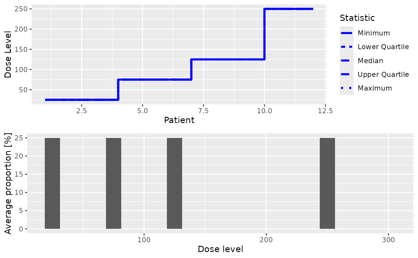
This plot method can be applied to GeneralSimulations objects in order to summarize them graphically. Possible types of plots at the moment are:

trajectory

Summary of the trajectory of the simulated trials

dosesTried

Average proportions of the doses tested in patients

You can specify one or both of these in the type argument.

Usage

# S4 method for class 'GeneralSimulations,missing'
plot(
  x,
  y,
  type = c("trajectory", "dosesTried"),
  prob_plot_type = c("lollipop", "bar"),
  dose_scale = c("auto", "linear", "log"),
  axis_ticks = c("dosegrid", "regular"),
  patient_scale = NULL,
  ...
)

Arguments

x

(GeneralSimulations)
the object we want to plot from.

y

(missing)
not used.

type

(character)
the type of plots you want to obtain.

prob_plot_type

(string)
for the doses tried plot, use a "lollipop" (default) or "bar" geometry.

dose_scale

(string)
for dose axes, use "auto" (default), "linear", or "log". Automatic scaling is linear except when equal-width bars would overlap, in which case the doses tried x-axis uses log10. The trajectory y-axis uses log10 only when explicitly requested. Log scaling requires all doses to be strictly positive.

axis_ticks

(string)
place dose-axis ticks at each dose-grid value ("dosegrid", the default) or at regular positions selected by ggplot2 ("regular"). This controls the trajectory y-axis and doses tried x-axis.

patient_scale

(numeric or NULL)
patient positions for the trajectory x-axis ticks. By default, the unique cumulative active-treatment cohort sizes are inferred from the simulation data. A single supplied value is used as an equally spaced interval; a vector supplies the exact breaks.

...

additional arguments without method dispatch.

Value

A single ggplot object if a single plot is asked for, otherwise a gtable object.

Examples

# nolint start

## obtain the plot for the simulation results
## If only DLE responses are considered in the simulations

## Specified your simulations when no DLE samples are used
## Define your data set first using an empty data set
## with dose levels from 25 to 300 with increments 25
data <- Data(doseGrid = seq(25, 300, 25))

## Specified the model of 'ModelTox' class eg 'LogisticIndepBeta' class model
model <- LogisticIndepBeta(
  binDLE = c(1.05, 1.8),
  DLEweights = c(3, 3),
  DLEdose = c(25, 300),
  data = data
)
## Then the escalation rule
tdNextBest <- NextBestTD(
  prob_target_drt = 0.35,
  prob_target_eot = 0.3
)

## The cohort size, size of 3 subjects
mySize <- CohortSizeConst(size = 3)
## Deifne the increments for the dose-escalation process
## The maximum increase of 200% for doses up to the maximum of the dose specified in the doseGrid
## The maximum increase of 200% for dose above the maximum of the dose specified in the doseGrid
## This is to specified a maximum of 3-fold restriction in dose-esclation
myIncrements <- IncrementsRelative(
  intervals = c(min(data@doseGrid), max(data@doseGrid)),
  increments = c(2, 2)
)
## Specified the stopping rule e.g stop when the maximum sample size of 12 patients has been reached
myStopping <- StoppingMinPatients(nPatients = 12) | StoppingMissingDose()
## Now specified the design with all the above information and starting with a dose of 25
design <- TDDesign(
  model = model,
  nextBest = tdNextBest,
  stopping = myStopping,
  increments = myIncrements,
  cohort_size = mySize,
  data = data,
  startingDose = 25
)

## Specify the truth of the DLE responses
myTruth <- probFunction(model, phi1 = -53.66584, phi2 = 10.50499)

## Then specified the simulations and generate the trial
## For illustration purpose only 1 simulation is produced (nsim=1).
## The simulations
mySim <- simulate(
  design,
  args = NULL,
  truth = myTruth,
  nsim = 1,
  seed = 819,
  parallel = FALSE
)


## plot the simulations
print(plot(mySim))



## If DLE samples are involved
## The escalation rule
tdNextBest <- NextBestTDsamples(
  prob_target_drt = 0.35,
  prob_target_eot = 0.3,
  derive = function(samples) {
    as.numeric(quantile(samples, probs = 0.3))
  }
)
## specify the design
design <- TDsamplesDesign(
  model = model,
  nextBest = tdNextBest,
  stopping = myStopping,
  increments = myIncrements,
  cohort_size = mySize,
  data = data,
  startingDose = 25
)
## options for MCMC
## The simulations
## For illustration purpose only 1 simulation is produced (nsim=1).
# mySim <- simulate(design,
#                   args=NULL,
#                   truth=myTruth,
#                   nsim=1,
#                   seed=819,
#                   mcmcOptions=options,
#                   parallel=FALSE)
#
# ##plot the simulations
# print(plot(mySim))
#

# nolint end